For me, coding is a heady combination of 🖋️ writing and
🧩 puzzle solving and ❤️ care. And sometimes the software ends
up being useful, too. 😄
Here are some of the projects I've worked on.
Theanets 📖
📖
theanets is a neural network toolkit for
Python that uses
Theano for the heavy
lifting. Thanks to Theano, your models will transparently run on a GPU.
The toolkit makes it easy to create a wide variety of machine learning
models, including linear dense and sparse autoencoders (e.g., PCA and ICA),
denoising autoencoders, linear and nonlinear regression, regularized
regression (e.g., lasso or elastic net), linear and nonlinear classifiers,
and recurrent autoencoders and classifiers, including models using LSTM
cells or Clockwork RNN layers.
Models can be constructed using different activation functions (e.g.,
linear, rectified linear, batch normalization, etc.) and different numbers
of layers (e.g., deep models). It is also easy to add different regularizers
to each of the models at optimization time—in fact, regularization is
often what differentiates two otherwise very similar models (e.g., PCA and
ICA).
import theanets, numpy as np

def sample(n): return np.random.randn(n, 10)

# create an autoencoder model.
ae = theanets.Autoencoder([10, 2, 10])

# train it with a sparsity regularizer.
ae.train(sample(1000), sample(100),
         algo='rmsprop', hidden_l1=0.1)

# continue training without the regularizer.
ae.train(sample(1000), sample(100),
         algo='nag', momentum=0.9)

# use the trained model.
ae.predict(sample(10))
Downhill📖
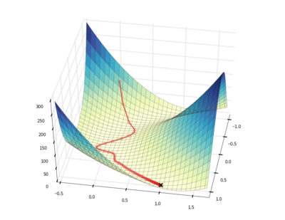
downhill is a collection of stochastic gradient optimization
routines for loss functions defined using
Theano.
The package implements vanilla stochastic gradient descent (SGD), resilient
backpropagation, RMSProp,
ADADELTA,
Equilibrated SGD, and
Adam. All optimization
algorithms can be combined with traditional and
Nesterov (PDF)
momentum.
import climate, downhill, theano, numpy as np
import theano.tensor as TT

climate.enable_default_logging()

def rand(*s): return np.random.randn(*s).astype('f')

# Set up a matrix factorization problem to optimize.
A, B, K = 20, 5, 3
u = theano.shared(rand(A, K), name='u')
v = theano.shared(rand(K, B), name='v')
e = TT.sqr(TT.matrix() - TT.dot(u, v))

# Create a noisy low-rank matrix to factor.
z = np.clip(rand(A, K) - 0.1, 0, 10)
y = np.dot(z, rand(K, B)) + rand(A, B)

downhill.minimize(
    # loss = |x - uv|_2 + |u|_1 + |v|_2
    loss=e.mean() + abs(u).mean() + (v * v).mean(),
    train=[y], batch_size=A, max_gradient_norm=1,
    learning_rate=0.1)

print('Sparse Coefficients:', u.get_value())
print('Basis:', v.get_value())
Pagoda
Combines the ODE physics simulator with some OpenGL tools for
visualization, and a simple grammar for defining articulated bodies.
import click, pagoda, pagoda.viewer, numpy as np

# Implement a custom world reset that randomly repositions things.
class World(pagoda.physics.World):
    def reset(self):
        for b in self.bodies:
            b.position = np.array([0, 0, 10]) + 3 * rng.randn(3)
            b.quaternion = pagoda.physics.make_quaternion(
                np.pi * np.random.rand(), 0, 1, 1)

# Helper for generating gamma-distributed random values.
def gamma(n, k=0.1, size=1):
    return np.clip(np.random.gamma(n, k, size=size), 0.5, 1000)

w = World()

# Create 100 bodies in the world -- random shape, size, and color.
for _ in range(100):
    shape, kwargs = sorted(dict(
        box=dict(lengths=gamma(8, size=3)),
        capsule=dict(radius=gamma(3), length=gamma(10)),
        cylinder=dict(radius=gamma(2), length=gamma(10)),
        sphere=dict(radius=gamma(2)),
    ).items())[np.random.randint(4)]

    body = w.create_body(shape, **kwargs)
    body.color = tuple(np.random.uniform(0, 1, size=3)) + (0.9, )

# Run the simulation!
w.reset()
pagoda.viewer.Viewer(w).run()